The true meaning of your zip code
Socioeconomic factors widen the playing field in all stages of life.
The harder you work, the more money you’ll make.
A phrase often shared around social circles and conversations, a tale only true for those who are lucky enough. People that grew up in financially disadvantaged households are frequently grieved with having to work multiple jobs just to make ends meet.
This problem is known all too well by hundreds of thousands of families across the United States.
According to a 2014 study by the Pew Research Center, 24% of Americans believed that the reason low-income citizens are still poor is due to their “laziness” and “employment status” but this perception isn’t true.
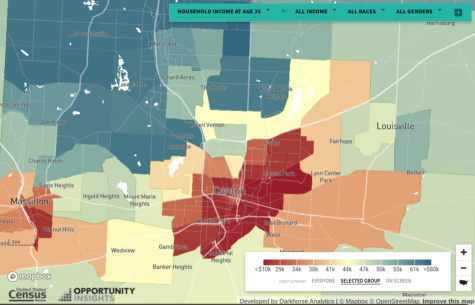
In 2014, a group of Harvard and Brown University researchers ran studies with the help of the United States Census Bureau. What they created was a map, which compiled data like household income, high school graduation rates, incarceration rates, and others, which in turn gave estimates for a child’s average income for when they grew up based on where they live.
The results were disheartening, it found that for every year that a child grows up in an area with a better “rating” on the Opportunity Atlas it greatly increased their chances of having a better outcome in adulthood and for every year that a child lives in an area with a worse “rating”, their chances greatly decrease.
Socioeconomic disadvantages can arise from, where a person grew up, or the median income of their parents, etc. For many families, these factors can force them into poverty, and when not addressed can trap the family in an endless cycle for generations.
It is important to note that success is subjective, and variables like wealth, education, access to healthcare, and affordable housing are all major factors in determining the likelihood of success in an individual.
Education
One of the many major puzzle pieces which can determine a child’s future outcomes, is the education that they receive. Public schools receive their funding on Local, State and Federal levels. They receive a bulk of their funding from property taxes, this can be different from school to school causing some to have more than others. The Federal Government aims to offset this disparity by providing federal aid to schools.
Schools in disadvantaged areas are often forced to play a game of catch up compared to their counterparts in areas with financially stable students. Researchers at the Institute for Research on Labor and Development comprised many theories on why schools with disadvantaged students often perform worse on standardized tests, state metrics, and performance measures than their advantaged counterparts. For example, they cite reasons like Teacher attrition, which may cause hindrance when attempting to hire the most qualified teachers.
Another reason cited is the general lack of resources, since schools are mainly funded by property taxes, schools in disadvantaged areas typically receive less money from their community. The researchers explain that this may cause schools to be ill-equipped and be unable to provide amenities to their students.
Another factor that can be a disadvantage is chronic absenteeism. It is defined as a student missing 10 or more days of school regardless of the reason. Chronic absenteeism is typically much more frequent in disadvantaged communities, as research suggests, this may be due to multiple reasons like poor health, lack of access to transportation, and lack of safety.
Comparison of Local High Schools(statistics available on Ohio Department of Education-Report Cards)
| GlenOak HS | McKinley HS | Hoover HS | Jackson HS | |
| Average Household Income | $51,537 | $32,735 | $60,473 | $81,357 |
| Average Spending per Pupil | $8,390 | $11,896 | $10,301 | $9,007 |
| Chronic Absentee Percentage | 13.4% | 56.1% | 20.4% | 5.5% |
| Percentage Spending on Classroom Instruction | 69.9% | 72.4% | 74.2% | 77.6% |
| ELA OST Proficiency | 69.7% | 30.2% | 85.8% | 80.4% |
| Math OST Proficiency | 38.7% | 7.3% | 65.4% | 66.2% |
| Graduation Rate | 95.6% | 84.4% | 95.9% | 98% |
| Ohio Performance Index(out of 120) | 74.0 | 41.7 | 93.1 | 89.6 |
One of the most interesting things about this graph is that McKinley Senior High School technically spends the most money per student out of the four schools, but overall performed the worst on all performance metrics. According to the study referenced earlier by the Institute for Research and Development, schools that are located in disadvantaged areas are forced to spend more money to level the learning playing field. The data from the table depicts a correlation between household income and education.
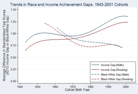
Graph by Stanford CEPA
According to a conference held at Stanford University with the Center for Education Policy Analysis, the gap in performance scores between poor and rich counterparts has been on a sharp increase since the 1980s.
In 2002, President George W. Bush signed the “No Child Left Behind” act, which authorized multiple federal programs that targeted the income gap and provided assistance for disadvantaged students. The bill greatly increased test scores nationwide and ensured quality education for underprivileged students. However, the bill largely failed because it penalized schools for scoring less than proficient on standardized exams but failed to reward the same schools for students who scored above the benchmark.
The bill was replaced in 2015 by the “Every Student Succeeds Act.” This act repealed penalties on schools for failed benchmarks. It also moved the power to the hands of the states.
Healthcare
Healthcare is a hot topic that bases its boundaries upon those who live in poverty and how that affects their health and their access to affordable treatment. In 2019, the uninsured population had risen to roughly 10.9%. According to the United States Census, 71% of Americans cite that the reason that they don’t have health insurance is because of how costly it is.
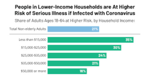
The COVID-19 Pandemic caused a small correlation between deaths and income status according to the Center for Disease Control. It can be inferred that this is the case due to the amount of economic and health situations that impoverished communities are challenged with. For example, low income workers often worked jobs that were labeled as essential during the pandemic, putting them at a greater risk of infection. Furthermore, low-income Americans without health insurance are less likely to go to the emergency room when experiencing life-threatening symptoms due to the fear of the cost.
There are many diseases which are much more common in low-income communities than in their middle and upper class counterparts. These diseases are called “diseases of poverty” and they include Asthma, Cardiovascular Disease, Dental Decay, etc. These diseases have dire consequences as living in poverty can not only increase your chances of contracting these diseases, but they can increase their severity.
Housing
Access to housing is one of the largest indicators of whether a cycle of intergenerational poverty will continue. According to Stanford Economist Raj Chetty, children who lived in communities with below average levels of poverty saw their average income increase by 31% in their adult life.
Reducing the levels of poverty is not just good for American citizens, it is also good for the government. Research completed by the National Low Income Housing Coalition found that on average, the American government loses around $2 trillion dollars each year due to low wages and productivity. These researchers also found that the American GDP would be around 13.5% higher than today’s if the government put effort into affordable housing.
Redlining
In 1933, as a part of Franklin D. Roosevelt’s “New Deal” the Home Owners Loan Corporation was created. In order to stimulate the housing market, HOLC sent out hundreds of surveyors and appraisers to communities all across the country. They graded communities on a 4-tiered report card, which was then handed to local private banks.
“Green” communities were the most ideal color for families. They had a high household income, with a thriving commercial sector, but there is one major flaw to this system. The presence of African-Americans or immigrants automatically reduced the color grades. For example, the “Blue” communities have almost identical traits to the green neighborhoods except that they have African-American centers in the proximity of the neighborhood.
“Yellow” communities were listed as “declining” according to HOLC. This was often due to the presence of immigrants. For the most part, these neighborhoods were low to middle class and were often given a low security grade based on stereotypes against immigrants.
“Red” communities were typically low-class neighborhoods which, according to HOLC, were defined as “hazardous”. There were minimal differences between the communities except for race and place of birth. Since the neighborhoods were labeled “red” the term redlining gradually gained recognition. Banks never approved loans and mortgages from families who resided in red neighborhoods under the guise that they were too risky to give loans to.
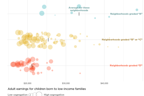
Redlining had lasting effects on African-Americans and low-income families to this day. According to the model above, redlining greatly decreased expected earnings amongst children who grew up in red or yellow neighborhoods.
Another effect is the changes in healthcare, redlining has kept many families in the cycle of intergenerational poverty. Many families who reside in the Red or Yellow neighborhoods were much more likely to be uninsured.
Historical Redlining involved the principle of denying families loans and mortgages solely based on their race or income. These same outlines of neighborhoods are still seen today, continually disadvantaging people solely based on their ZIP code.
Although ZIP codes are not solely responsible for success, it would be foolish to deny the impact they have. Until solutions are signed into law that minimize the effects of socioeconomic status on success, the United States will continue to experience wider gaps in economic disparities.
Sources
Ohio School Report Cards. (n.d.). Retrieved March 28, 2022, from https://reportcard.education.ohio.gov/
Geoffrey T. Wodtke, Ugur Yildirim, David J. Harding, and Felix Elwert. (2020). “Inequality of Educational Opportunity? Schools as Mediators of the Intergenerational Transmission of Income”. IRLE Working Paper No. 102-20. http://irle.berkeley.edu/files/2020/05/Are-Neighborhood-Effects-Explained-by-Differences-in-School-Quality.pdf
Neighborhoods. Opportunity Insights. (2019, August 5). Retrieved March 29, 2022, from https://opportunityinsights.org/neighborhoods/
Income, inequality, and educational success: New evidence about. Center for Education Policy Analysis. (n.d.). Retrieved March 29, 2022, from https://cepa.stanford.edu/iies2012
Hotez, P. J. (2008, June 25). Neglected infections of poverty in the United States of America. PLoS neglected tropical diseases. Retrieved March 29, 2022, from https://www.ncbi.nlm.nih.gov/pmc/articles/PMC2430531/
The opportunity atlas. The Opportunity Atlas. (n.d.). Retrieved March 29, 2022, from https://www.opportunityatlas.org/
The problem. National Low Income Housing Coalition. (n.d.). Retrieved March 29, 2022, from https://nlihc.org/explore-issues/why-we-care/problem
The lasting impacts of segregation and redlining. SAVI. (2021, June 24). Retrieved March 29, 2022, from https://www.savi.org/2021/06/24/lasting-impacts-of-segregation/
Your donation will support the student journalists of GlenOak High School. Your contribution will allow us to purchase equipment and cover our annual website hosting costs.
Dylan Wolfe is a senior at GlenOak High School this year. This will be his second year on staff. Dylan is involved in Academic Challenge, Ohio Model United...